Introduction

MATLAB is a powerful computing environment that is used in a variety of fields including mathematics, signal processing, financial modeling and statistical analysis. The content of this class covers only a narrow scope of MATLAB’s computational capabilities, but demonstrates many of the tools used in more advanced applications.

About this Class

This class is an extension of MATLAB 1 that focuses on a single, complex application: the graphical simulation of a forest fire. This is accomplished using programming tools both new to this course and those introduced previously.

Prerequisites

• A general knowledge of computers.

• MATLAB 1 or equivalent programming experience.

Other requirements

To use this manual, you will need a copy of the MATLAB 2 class files. These files can be found at “www.wisc.edu/sts”.

The required files are:

• forest_setup.m

• forest.m

• forest_finished.m

• neighbors_on_fire.m

Getting Started

1. Copy and paste the folder containing the class files to a location of your choice.

2. Open the MATLAB Environment and familiarize yourself with the interface.

3. Navigate to the directory panel on the left and change the current directory to the location in which you have saved a copy of the class files.

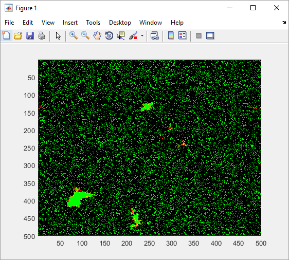
4. In the command window,type forest_finished and press enter.

This will run a completed script to give you a preview of the final product. A small window should pop up showing what appears to be a pixilated, animated aerial view of a forest fire (see below).

Forest Fire Simulation

Class Files

A file called forest_setup.m has already been created for you. It contains variable assignments which allow us to use numeric values for the color and state of the vegetation repeatedly with a simple name.

In other words, instead of remembering that the number 1 represents a patch with low vegetation, we can use the variable low_veg. The variables in our simulation range from 1 (low vegetation) to 7 (ash). The advantage of using this naming scheme of variables is that it will make our code much easier to write and read, and the colors can be easily changed.

A file called forest.m has an outline of what we will do today, called a “skeleton” of code. We will fill in what we need step by step. The top section sets up the parameters of the forest. The bottom section will do the simulation.

neighbors_on_fire.m implements the computer logic needed to determine whether a particular patch of forest has a neighboring patch that is on fire. This code is beyond the scope of this class, so we will simply take for granted that it works correctly and use it later as needed.

About the Forest

The forest is an animation in which each new “frame” is determined by a set of rules. The rules take what the forest looks like in the current frame and use the information to compute what the next frame should look like. The goal of this class is to translate these rules into computer logic so that MATLAB can produce the animation we want.

The forest is made of many individual patches, each of which can exist in seven possible states:

• Growing: low vegetation state, mid vegetation state, high vegetation state

• Burning: high fire state, mid fire state, low fire state

• Ash state

During each cycle of the simulation, states progress as follows:

• Low vegetation always progresses to mid vegetation

• Mid vegetation always progresses to high vegetation

• High Fire always progresses to mid fire

• Mid fire always progresses to low fire

• Low fire always progresses to ash

The two tricky states are the high vegetation and the ash state:

• High vegetation will occasionally be struck by lightning and ignite

• High vegetation will occasionally ignite if one of its neighboring patches is on fire

• Ash will occasionally grow into low vegetation

Parameters of the Simulation

Parameters are the numbers we use to tell MATLAB the properties of the system, specifically the size of the forest and how it should look when the simulation begins.

How often high vegetation catches fire and how often ash turns to vegetation can be defined using the idea of probability. If we specify a probability for each of those events, we can later use that to determine how a particular patch should progress.

Initializing the Simulation

Loading in variables

The forest simulation uses a group of variables

1. Enter close all and clear all at the top of the forest.m script

   This will clear out any old variables or graphs you may have left over from previous programs.

2. Enter forest_setup to setup the variables for the simulation.

Forest Size

We first need to determine the size of the forest. In programming, it is good practice to name any special numbers with a variable, especially if you plan to use it repeatedly or change it later. Let’s start off our code by defining the size of the forest. We will make it a square forest, that is, the sides will both be the same length. For this reason, we only need to store one number as a variable for forest size.

1. Enter forest_size = 500; in the forest.m file.

Recall that the semicolon suppresses output to the command window.

Specifying start states

We also need to specify the possible starting states, or initial conditions, for the patches in the forest. That is: do we want the whole forest to start as ash, low vegetation, something else, or some combination?

Recall from MATLAB 1 that an array is a systematic way for MATLAB to store data in two dimensions. You can visualize this as a table, where each cell corresponds to a unique position in the table, specified by row number and column number. This array, which will begin as a collection of start states and then cycle to different states according to our rules, will ultimately be used to create an animation.

Suppose we want the forest to begin such that any particular patch is either low vegetation, medium vegetation, or high vegetation on a purely random basis

1. Recall Possible States

We have three possible choices for starting our forest: low, medium, or high vegetation. If you look in forest_setup.m you can see that these states are the first 3 values in the states array. Therefore we can use MATLAB’s built in random integer generator function, randi, to start our new forest array with one of those three values: in other words, a random integer less than or equal to 3.

2. Create and Populate a New Array

Create an array of the specified size and populate it with values chosen randomly from integers less than or equal to 3. This can be accomplished with the function randi, where the first “argument” between the parentheses is the upper limit of integers we can choose from, and the values inside the brackets correspond to the dimensions of the forest array.

3. Enter forest = randi(3, [forest_size, forest_size]) in your script.

Using Probability to Determine New State

We can later use this idea of selecting randomly to our advantage by incorporating probability. If we define what probability a patch of ash has of turning into new vegetation, we can determine which ash patches are “lucky” by assigning each one a random value and comparing that to the probability.

For example, if we say that some ash has a 30% chance of turning into vegetation, we can assign each patch of ash a random number between 0 and 100, and any patch which ends up with a number less than or equal to 30 is “lucky” and turns into new vegetation. All others remain as ash.

For now, all we have to do is define these probabilities as variables. We’ll use them later. Let’s say that the probabilities are as follows:

• Probability of high vegetation being struck by lightning: 0.001%

• Probability of high vegetation catching fire from neighboring patch: 25%

• Probability of ash turning to low vegetation: 0.1%

Feel free to use your own numbers.

Filling in the Code

The probabilities simply need to be filled out. The names are already specified for you, because some of the class files require those exact names to work.

%Probabilities
  probability_of_lightning = .00001;
  probability_of_spread = .25;
  probability_of_growth = .001;

Drawing the Forest

To visualize the forest, we will use the image function. The function creates a graph and displays one square for each value in the matrix. The color of the square is determined by the value of that position in the matrix.

1. Enter img = image(forest);

The right hand side of the equation will create the graph. Once the graph is created, it assigns a handle (or a reference) to the variable on the left, img. We do this so that we can later refer to the graph using the variable img.

We now have an image of the forest, but the colors are not representative of the patches. We can adjust what value (or in our case state) relates to which color through the use of the colormap function. The color map function requires a list of colors (in a column) that will correspond to a value. The list of colors increases from 1 to the maximum value of the matrix (in our case, 7). That means that we need to specify 7 color values. MATLAB understands colors numerically (as RGB values), so for convenience, forest_setup.m has created variable names for the colors we will use.

2. Enter forest_setup.m and Enter the following code:

map = [light_green; mid_green; high_green; yellow; orange; red; black];

Once we’ve created the map, we can pass the map to the colormap function.

3. Enter colormap(map);

Control Logic

Boolean Logic and If-Statements

As you may recall from the data types discussed in MATLAB 1, Boolean data can only hold one of two possible values: true or false. This idea can be used in computer language so that certain parts of code will only execute if a particular set of conditions is true or false.

Guessing Game

As a simple demonstration of this, let’s play a guessing game with MATLAB, similar to the guessing game you may have played as a child. You will choose a number and assign it to a variable. Then we will have MATLAB generate a random number and assign it to a different variable. MATLAB can perform a simple test to see if the two are equal. If the result of that test is true, we will display a congratulatory message in the command window. It will be easiest to do this by creating a new script to contain the code.

1. Create a new script called guess.m

2. Pick Numbers and Assign Them to Variables

guess = 5;
    truth = randsrc(1,1, [1:10]);
    truth = randi(10, [1,1]);
    truth= 10*rand(1);

3. Use Boolean Operators and If-Statements to Decide Output

if (guess==truth)
    display(‘Congratulations!’);
end
if (guess ~= truth)
    display(‘Try again.’);
end

Advanced Boolean Operators

Other Boolean operators will be used in the forest fire to determine whether a condition is true or false. Feel free to experiment with the following.

Less-Than/Greater-Than Operators

1. The less-than operator tests if the first value is less than the second value.

   • 1 < 5 is true

   • 7 < 2 is false

2. The greater-than operator tests if the first value is greater than the second value.

   • 1 > 5 is false

   • 7 > 2 is true

AND/OR Operators

1. The AND operator tests to see if all conditions listed are true.

   • 1 < 5 && 2 < 7 is true

   • 1 < 5 && 2 > 7 is false

2. The OR operator tests to see if any of the conditions listed are true.

   • 1 < 5 || 2 < 7 is true

   • 1 < 5 || 2 > 7 is true

Application

We will be using if statements to direct the progression of the forest. That is, we want different things to happen depending on what state a given patch is in. We know that the high_veg and ash states are going to be special states, so they will each have their own section (using an if and elseif). The rest of the states will be treated the same, so they can all go in the else. We can make the general outline now and then we will fill it in as we learn more.

1. Enter the following code in the forest.m script.

if (state == high_veg)  %deal with the high vegetation state
elseif (state == ash)  %deal with the ash state
else %deal with the other states
end

Loops

For-Loops in MATLAB

A loop is another control structure that repeats a segment of code a certain number of times. MATLAB’s loops are different from other languages in a few crucial ways.

A MATLAB loop just cycles through values in an array. So for instance, if we have an array with five values in it, the loop will occur five times. During each of cycle of the loop, the loop variable will be assigned one of those values.

For example:

prime = [2 3 5 7 11];
for ii = prime
    display(ii)
end

This example will print out the values of the array prime. During each cycle, the next value of the array is passed to the ii variable.

People often use i and j as the loop variables (traditionally, i and j are used; but in MATLAB, i and j are the imaginary number sqrt(-1)). Some people use m and n in MATLAB.

More commonly, people will create the array directly in the for statement. For example:

for ii = 1:20
    display(ii)
end

Remember, that the colon operator is used to fill an array. In this case, the array has number from 1 to 20 (the increment valued is assumed to be 1 if it isn’t specified).

Vectorization in MATLAB

Loops are a necessary tool in all languages, but some practices (and ways of thinking) with loops don’t work well in MATLAB. For instance, in other languages, the way to simulate our Forest Fire would be to loop through every patch and then adjust its state. That is not the optimal way to use loops in MATLAB.

Since MATLAB is built to be a matrix language, it relies upon the idea of vectorization to be fast. Vectorization is the process of preforming operations on a vector of values all at once.

A simple example of this can be seen if you want to find the difference between each value in an array (maybe to check for duplicates, for instance).

array = randsrc(100,1,[1:10]); %creates an array of 100 random values
array = randi(10,[1,1]);
for ii = 2:length(array) %will go through every value of the array
    minus_prev_array(ii-1) = array(ii) – array(ii-1);
end

The indices of the arrays have to be adjusted to ensure that there is no error. However, this entire loop can be condensed (and optimized) by using the built in function diff.

minus_prev_array = diff(array);

Whenever you are using a loop in MATLAB, make sure that there is no way to vectorize. We still do need to make use of a loop in our simulation though. But instead of looping through the patches of the forest, we will loop through the different states of the forest (only 7 values). We can pass each of those states then to the if statement that we already set up.

Let’s see how this will work.

for state = fliplr(states) %take each state (one at a time)
    %Code created earlier
end

Finally, we will also use a loop to determine the number of cycles we want in our simulation. This loop will surround the loop we just created.

num_cycles = 100;
for ii = 1:num_cycles  %our code so far
end

Logical Indexing

As we’ve seen, MATLAB has more efficient tools than using loops. One of the most useful is the idea of logical indexing (LI). We can make use of logical indexing in our forest example. The idea of LI is that you can selectively manipulate values of a matrix. In our example, we will want to select all of the patches of the matrix that our in the low_veg state and transform them to the mid_veg state.

To use logical indexing, you need to have some Boolean equation. In our case, that could be forest == low_veg. The return of that Boolean equation will serve as our indices. In other words, forest(forest == low_veg) will return every patch in the forest that is in a state of low vegetation.

Application

Vectorization to Change State of Every Patch

Let’s add in the code. Remember, this will go in the else statement, since we are only dealing with the easy states (not the high_veg or the ash state).

1. For “normal” cases, progress to next state in cycle

Let’s add in the code. Remember, this will go in the else statement, since we are only dealing with the easy states (not the high_veg or the ash state).

forest( forest == low_veg) = mid_veg;
forest(forest == mid_veg) = high_veg;

We can generalize this code further to have it encompass all of the different states (except for the high_veg and the ash state), as we loop through them. Remember that the loop variable (state) will take each of those values.

forest(forest== 1) = 2;
forest(forest ==2) = 3;
forest( forest == state) = state + 1;

2. Use probability to determine next state for special cases

We can also use logical indexing to deal with the ash and high_veg states. But since these involve a probability, we will need to use multiple logical statements.

One way to get something with a certain probability is to generate a random number (between 0 and 1) and see if that random number is below your probability. You may recall this principle from earlier.

For example:

  if rand < .75
       display(‘Success’);
  end

Approximately three out of four times, when you run that it will display ‘success.’ When we are dealing with the ash, we will use the same principle that we just saw to find which ash patches will regrow to low_veg.

In English, we want to find every patch that is ash and has a value less than the probability of regrowth and make that low_veg.

We know how to do this without the probability section.

  forest( forest == ash) = low_veg;

We can add in the probability, by using a big random matrix (and again seeing where it is below the probability value).

  rand(size(forest)) < probability_of_regrowth;

The rand function creates a matrix of the size of the forest.

To find where both of those statements are true, we can use the & statement.

A single & instead of the dual && works as an element-wise comparison. It is the same idea as dot-operator.

Dot operator recap:

• matrix^2 does matrix multiplication

• matrix.^2 squares each element

forest(forest == ash & rand(size(forest)) < probability_of_regrowth) = low_veg;

The high_veg state has two components to it. We need to check if any neighbors are on fire or if it gets struck by lightning. We know how to check if it is struck by lightning, because it is the same process of being regrown from ash.

forest(forest == high_veg & rand(size(forest)) < probability_of_lightning) = high_fire;

The next step is similar, but we need to check if any neighbors are on fire (and then again, include the probability section). To check if the neighbors are on fire, we will used a prewritten function (by the instructor) called neighbors_on_fire. This function creates a matrix that can be used as a logical index (the same way that rand(size(forest)) < probability does). So, this time we need to combine three matrices to form the logical index. We need the forest == high_veg and the rand(size(forest)) < probability_of_spread and the neighbors_on_fire matrices.

forest( forest == high_veg & rand(size(forest)) <
 probability_of_spread & neighbors_on_fire(forest)) = high_fire;

Animation

We now have our simulation. But if we were to run this, the graph would not update at all (in fact, it would freeze for a while and then start working after our program completed). To animate the graph, we need to explicitly state this.

To do this, we can update the color information of the image (because the color is the only thing that is changing, not the size). Remember that earlier we assigned our image to the variable img; we will now be able to use that variable to update the graph.

  set(img, ‘CDATA’, forest);
  drawnow

The set function is used to change the properties of an object (in our case of the graph). We want to change the CDATA property, which contains all of the color information.

Wrapping it Up

The final addition to our simulation will be an option to stop the simulation. We can have the simulation continue infinitely with something called a while loop. A while loop is a combination of a for loop and an if statement. It will continue to loop, until the condition is no longer true. In our situation, we can ask (after every set of 1000 cycles) if the user wants to quit.

To add in this while loop, we can surround all of our simulation code with the following statements.

while quit ~= ‘y’
%all of our code
end

Now our code will continue to function as long as the quit variable does not equal ‘y’. This means that we first need to set the quit variable to something other than ‘y’ and then we need to ask the user if s/he wants to quit.

quit = ‘n’
while quit ~= ‘y’
%our code
quit = input(‘Do you want to quit? (y/n)’, ‘s’);
end

Conclusion

MATLAB has a tremendous amount of applications from biology to aerospace. The best way to learn is by doing. So explore implementing MATLAB in your field. If you ever encounter difficulties, there are many resources online and individual Ask-A-Trainer consultations are available through STS.