R/RStudio 1
Introduction to Statistical Analysis
Introduction
What is R and what is it used for?
R is a free, open-source software and programming language developed in 1995 at the University of Auckland as an environment for statistical computing and graphics. R is a free, open-source software that is widely used in data analysis, statistical modeling, and graphical visualization of data.
R provides a wide range of statistical and graphical techniques for data analysis, including linear and nonlinear modeling, hypothesis testing, time series analysis, clustering, and more. This is further supported by a large ecosystem of packages contributed by a vibrant community of statisticians, data scientists, and researchers, which extends its functionality for various specialized tasks.
RStudio is a popular integrated development environment (IDE) for R, designed to provide a user-friendly interface for writing, running, and debugging R code. Together, R and RStudio provide a powerful and flexible environment for data analysis, statistical modeling, and visualization.
Why R/RStudio?
R and RStudio are popular choices among data scientists, statisticians, and researchers for several reasons besides those previously stated:
- Reproducible research: R has strong support for reproducible research, allowing users to create dynamic and interactive reports using tools like R Markdown and Shiny. These tools enable researchers to document their analyses, share their findings, and create reproducible reports that can be easily updated as data or analysis changes.
- Active and supportive community: R has a large and active community of users and developers who contribute to its development, create and maintain packages, and provide support through forums, mailing lists, and online resources. This community ensures that R remains up-to-date with the latest statistical techniques and best practices, and provides a valuable resource for learning and troubleshooting.
- Open-source and free: R is an open-source software, which means it is freely available to use, modify, and distribute. This makes it accessible to a wide range of users, from individual researchers to large organizations, without the need for costly software licenses.
It's important to note that the choice of programming language depends on the specific needs and requirements of the task at hand, and different programming languages may be better suited for different use cases. However, R's strengths make it a popular choice for many data scientists, statisticians, and researchers (and our school!).
Setting up R and RStudio
If you haven’t already done so, make sure you install both R and RStudio before we start with the class.
In order to download R, you can go to https://repo.miserver.it.umich.edu/cran/ and download R for the first time. This page is also useful since you can easily find the R manual here as well, which might prove to be useful once you start working on your own applications.
In order to download RStudio, you can go to https://rstudio.com/products/rstudio/download/ and download the free version of RStudio on your own machines. Follow the steps in the wizard and open up RStudio.
Introduction to the R Environment
Before opening our class files, we are going to go over a few essential RStudio functions.
Once open, your RStudio should look like this:
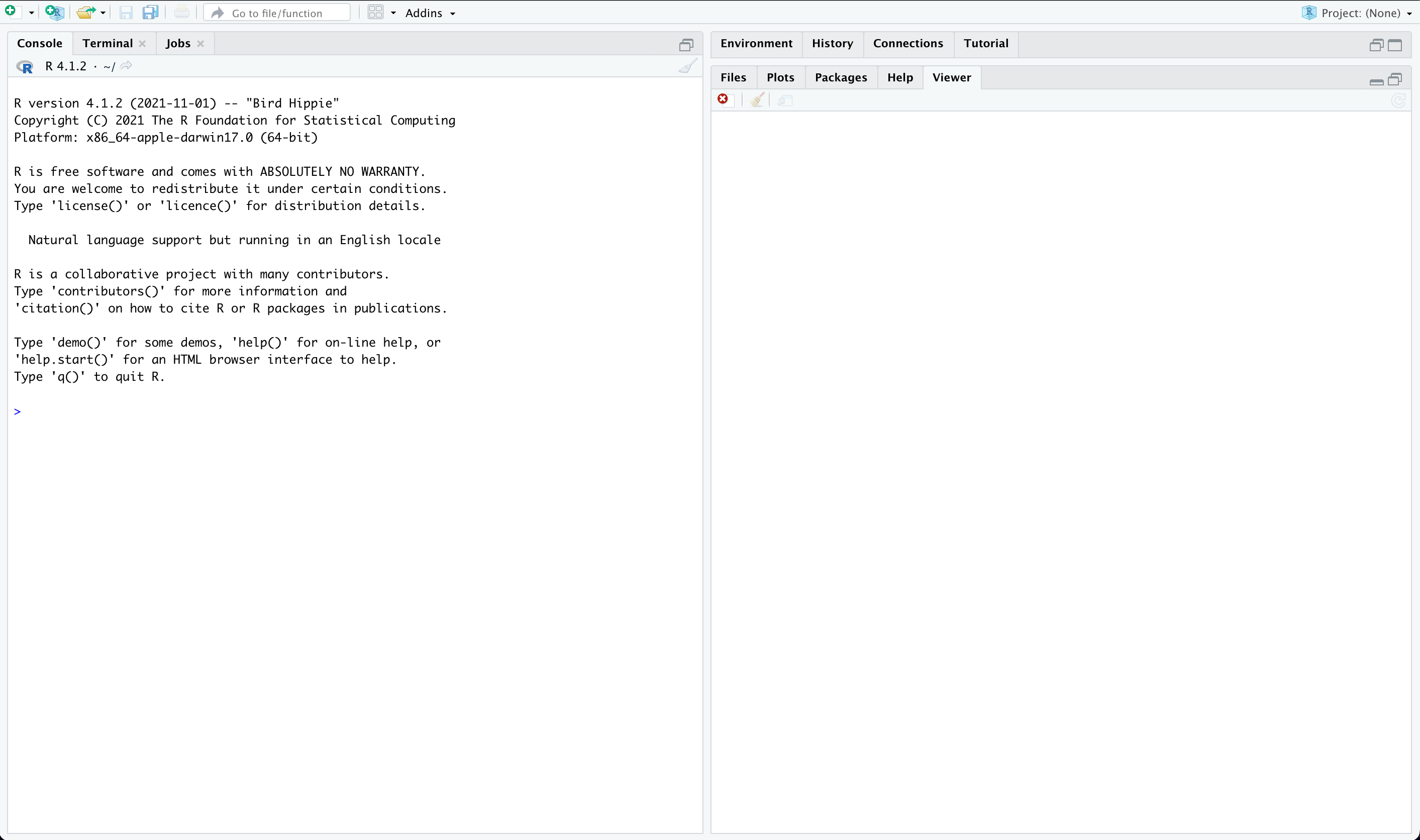
- Console: The console is the command-line interface in R where you can enter and execute R commands.
- Help Page: R has an extensive built-in help system that provides documentation and information about various functions and packages. You can access the help pages using the ? or help() function, which provides detailed information about the usage, arguments, and examples of a specific function.
- Environment Tab: The environment tab in RStudio provides a visual representation of the objects and data currently in your R environment. You can view, explore, and manipulate objects in the environment tab, which can be helpful for managing your workspace during data analysis.

- Enlarging/Shrinking Windows: RStudio provides buttons to easily resize or hide/show different panes such as the console, help page, and environment tab. You can customize the layout of your RStudio interface to suit your preferences and workflow.
R Markdown (RMD) files in R
R Markdown is a markup language that allows you to create dynamic documents that combine text, code, and visualizations. An RMD file is a plain text file that uses Markdown formatting to create a rich document with embedded R code chunks. RMD files are a popular format for reproducible research and can be used for creating reports, presentations, websites, and more.
In order to open the RMD file we will be working with today, go to File > Open File. From there, find the file ‘r-class-files.Rmd’ and select it.
Once done, you should have a screen that looks like this:
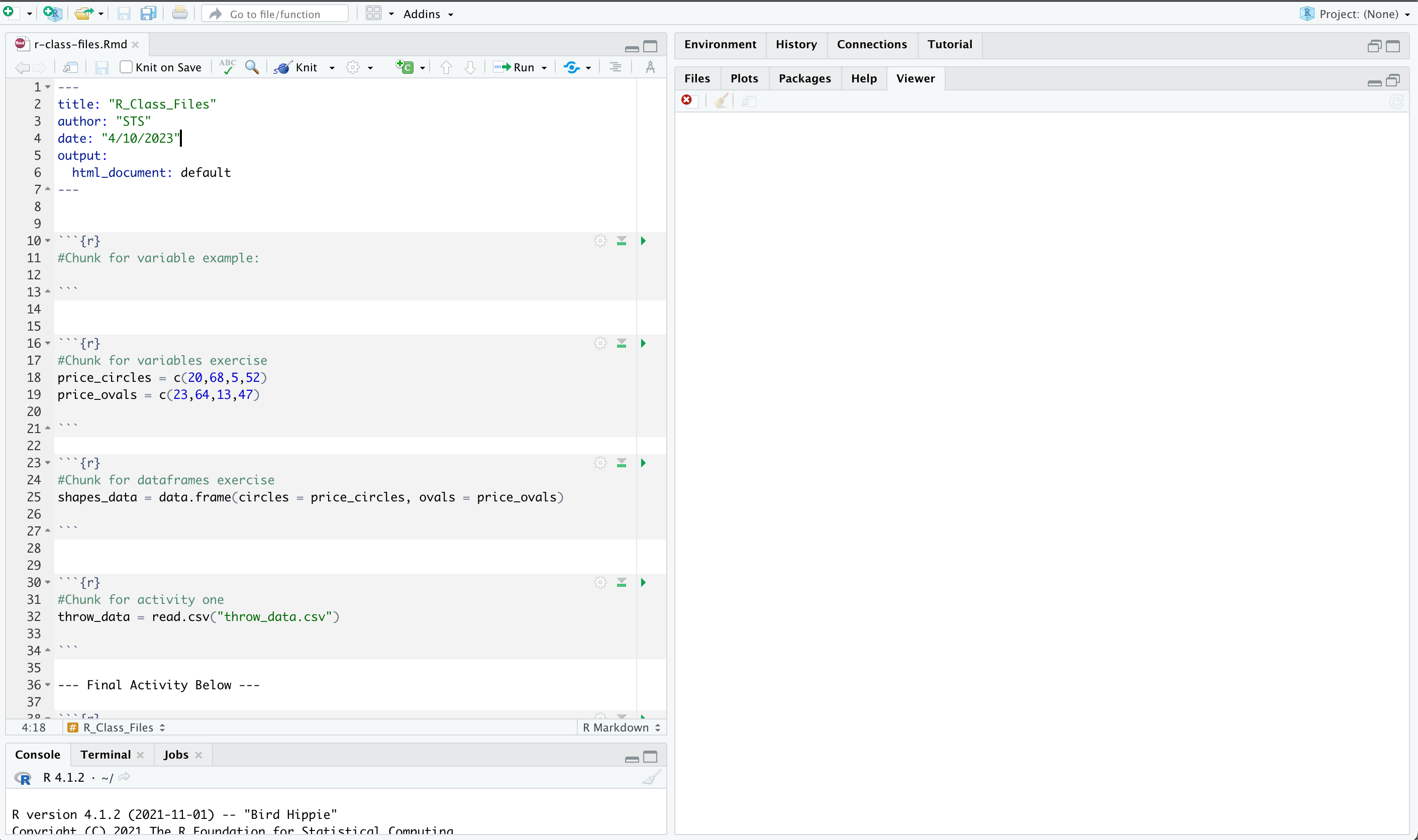
In an RMD file, code is organized into chunks, which are delimited by ```{r} at the beginning and ``` at the end of the chunk. R code chunks are where you can write and execute R code within your RMD file. You can include multiple code chunks in an RMD file, and each chunk can have its own set of options and parameters.

To run individual chunks in an RMD file, you can use the "Run" button in RStudio, which is located in the top right corner of each code chunk. Alternatively, you can use the keyboard shortcut Ctrl+Shift+Enter (Windows/Linux) or Cmd+Shift+Enter (Mac) to run the current chunk.
Running individual chunks allows you to test and debug your code in smaller pieces, making it easier to identify and fix any errors or issues. You can also control the order in which the chunks are executed by specifying chunk options such as eval and include (inside the {r} at the start of each chunk), which determine whether a chunk should be evaluated and included in the final output.
Knitting is the process of compiling an RMD file into a final document format, such as PDF, HTML, or Word. When you knit an RMD file in RStudio, it evaluates the R code chunks, generates the output, and combines it with the text and formatting to create a final, polished document that can be shared or published. You can knit an RMD file by hitting the ‘knit’ button near the yarn ball right above your code.
Variables
Variables are symbols or names that can be used to store some data inside them. In R, you can store a number as well as a list of numbers inside one variable name. There are 2 ways that you can initialize or assign a value to a variable in R:
			variableName = value
			variableName <- value
While these 2 signs look different, they are doing the same thing right now. Let's start by initializing two variables in our first chunk and running it:
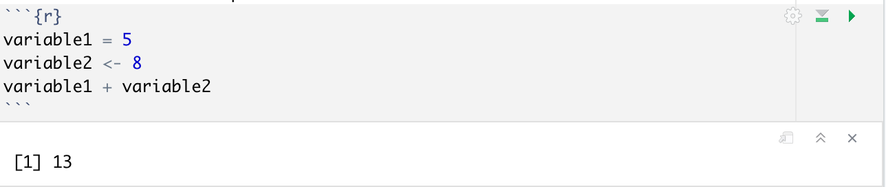
Notice how the variable assignment did not give any output, since R is storing these variables internally and not doing anything with them right now. You can store text data in a variable using the standard quotation marks, as well as boolean values(TRUE or FALSE values).
Remembering the environment tab from earlier, now that we have saved variables you can actually view them there! These values will also change as you change the values in your variables.
Vectors
A vector in R is a list of multiple values that are all of the same type. Doing so allows you to hold multiple values inside the same variable.
The way to make a vector is as follows:
vectorName = c(num1,num2,....)
For example, the vector c = c(1,2,3) gives us a vector c with 3 different values. In a vector, each element is delimited by a comma. In order to obtain a specific value from our vector, we can use the index of the item. Indexing in R starts from 1, which means that the first item will have index 1. We can get element of index i using the syntax
vectorName[i]
You can also obtain a subset of values from your original vector.
vectorName[a:b] will give you a subvector with values from index a to b
vectorName[c(a,b)] will give you a subvector with only values from index a and b
The c() function also has the ability to combine 2 vectors into one large vector. For example, if v1 = c(1,2,3) and v2 = (4,5,6) then c(v1,v2) gives us a vector (1,2,3,4,5,6)
R has some default functions for vectors, such as:
| max(x) | Get the maximum value of x |
| min(x) | Get the minimum value of x |
| range(x) | Get a vector which contains the max and min values of x |
| length(x) | Get the number of elements in x |
| sum(x) | Get the sum of all elements in x |
| mean(x) | Get the mean value of all elements in x |
| sd(x) | Get the standard deviation of x |
| var(x) | Get the variance of x |
| sort(x) | Sort the elements of x |
| quantile(x) | Gives the 0th, 25th, 50th, 75th and 100th percentiles for the data in x |
| summary(x) | Gives the quantiles as well as the median and mean of x |
Vectors also make it easier to perform calculations. All the basic arithmetic operators can be applied on a numeric vector. Adding two vectors v1 + v2 gives us a new vector which contains the sum of values from the same index.
You can also perform these arithmetic operations with a scalar value. For example, v1 + 2 gives us a new vector with all the values of v1 added by 2
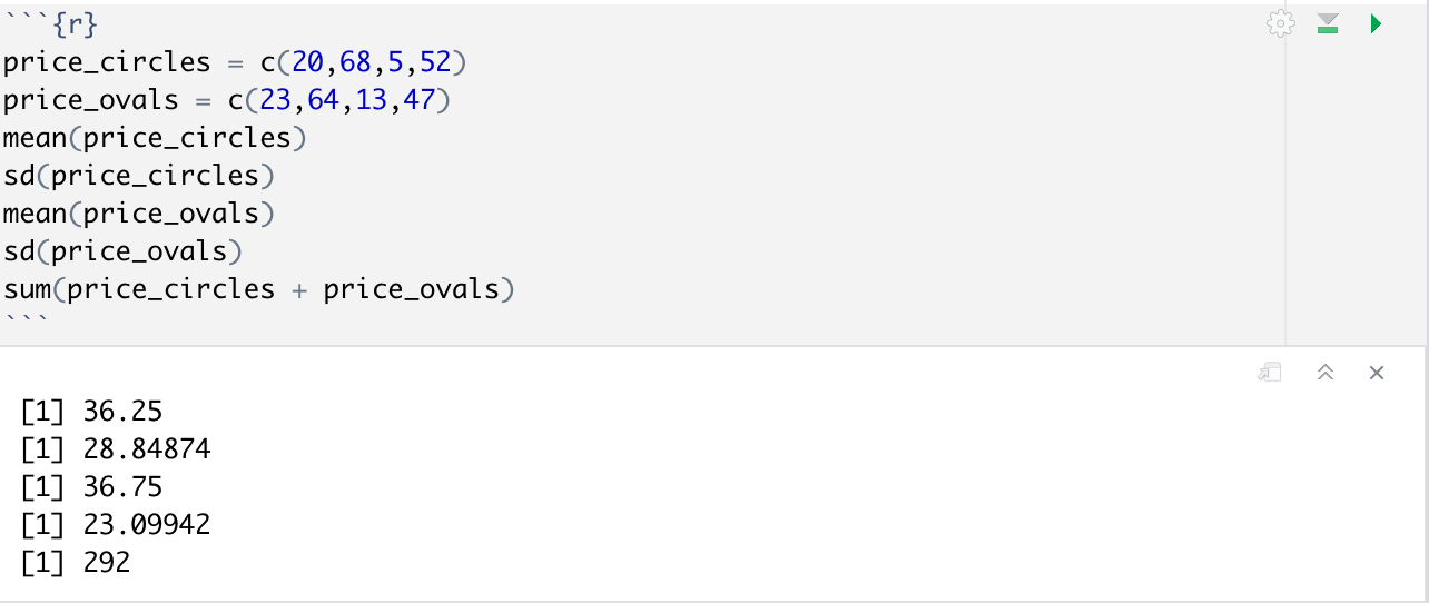
Exercise
Given a vector for the price of circles = c(23,64,13,47) and a vector for the price of ovals = c(23,64,13,47), compare the means and standard deviations of both as well as finding the cost of all ovals and circles combined.
DataFrames
While vectors are a simple way for us to allocate a set of data inside a variable, this may not be enough in some cases. For example, we would have to make a variable for an individual row or column for data taken from a table. There are 2 ways we can allocate a set of data in 2 dimensions:
In this workshop we will only be discussing DataFrames as they are much more common and widespread, but matrices still have their uses.
A dataframe is the most common way of storing some data in a table. A data frame is a table or a two-dimensional array-like structure in which each column contains values of one variable and each row contains one set of values from each column.
Building our own DataFrames
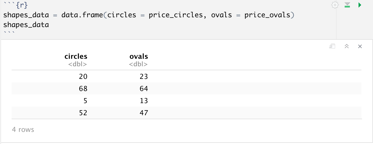
To create a dataframe, we can use the data.frame() function. Dataframes are initialized by providing a set of column names for our dataframe, which we can later use to add our data by its respective columns.
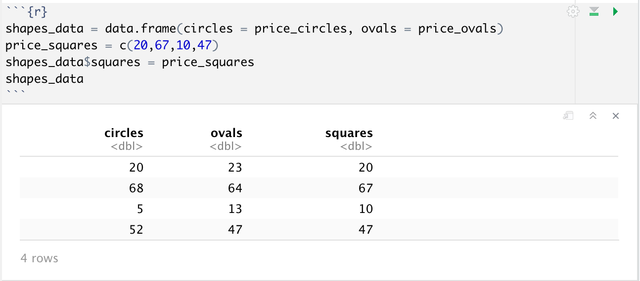
But what if we had data for a new shape, say squares, and wanted to add it to our dataframe? Luckily R makes it very easy for us to do this, provided our new data is the same length as our dataframe. All we have to do is df_name$column_name = new_column. The same $ operator can be used otherwise to select a single column from a dataset to work with, for example you could do mean(shapes_data$ovals) to get the mean price of ovals.
Importing DataFrames
You can import data into R from various sources, including libraries, CSV files, Excel files, and more. R provides built-in functions for reading data from different file formats, such as read.csv() for CSV files, read_excel() for Excel files (using the readxl or openxlsx package), and readr::read_delim() for other delimited files. You can also use packages such as tidyverse or data.table for more advanced data manipulation tasks.
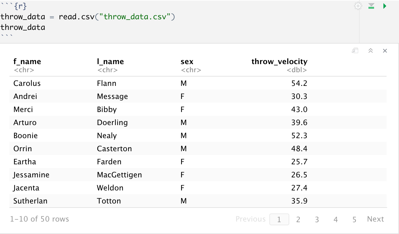
Most work you will have to do in RStudio will involve importing data to work with, so we will not be using the previously created DataFrame. For this workshop, we will be working with a csv file of some sample data for a class of 50 first-grade students, with their names, their biological sex, as well as the recorded horizontal velocity of the thrown ball.
Working with DataFrames
Indexing for a row can be done using the variableName[rowIndex, ] format. However, we can refer to a column using either its index or its name. Indexing by column number can be done using the variableName[rowIndex, colIndex] format. However, indexing by column name can be considered very useful if we are dealing with a larger dataset where it can be difficult for the user to always keep track of the column numbers. Indexing by column name can also make it easier for people to read and understand the code in an easier way. Indexing by column name can be done by the variableName$colName format, which returns a vector of the entire column.
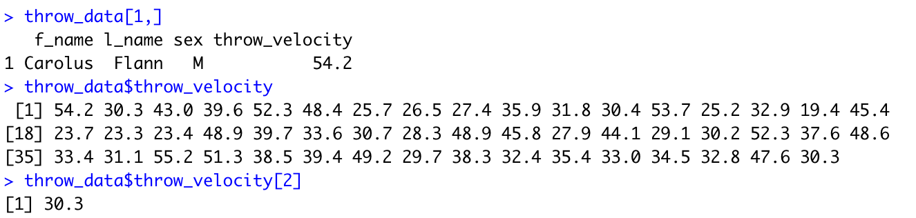
NOTE: The console is used here instead of chunks for readability, but the code is the same.
Note that sample[1] and sample[,1] gives us column 1, but sample[1,] gives us row 1. Try experimenting to grab different values from throw_data with indexing!
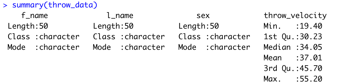
One of the most useful functions to use with dataframes is the summary() function. This function will provide some basic statistical information for each column of our dataframe, such as minimum/maximum values, mean, median, 1st quartile and 3rd quartile values.
While our dataframes will generally have a comprehensive table of values, it could sometimes be useful for us to obtain a subset of our former data. In R, we can use logical subsets in order to filter out some of our data. Generally we can do so by comparing a set of values in our dataframe to another value. We can perform comparisons based on measures of equality using any of the following syntax.
| == | Equal to |
| != | Not equal to |
| > | Greater than |
| >= | Greater than or equal to |
| < | Less than |
| <= | Less than or equal to |
NOTE: == and = do different things. = performs an assignment and == makes a comparison between 2 different values
For example, let's use our throw_data dataframe. Let's say we want a subset of all the students that are biologically male.
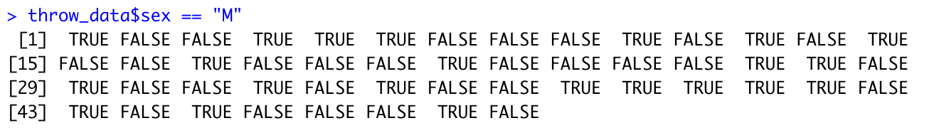
Note that we get a list of True/False values that correspond to all rows in our dataframe. All the values that are TRUE correspond to the indexes of values that satisfy the condition that we have set. Also note that this condition gives us a TRUE value when our value was also equal to “M”, so make sure to write your comparisons appropriately. In order to get the subset of data, we can use the following syntax to get a logical subset:
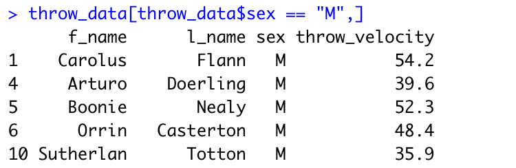
NOTE: Most of the rows printed are cut out for readability, there should be many more if you run it yourself.
R also allows you to use the subset(dataframe, criteria) function. The commandsubset(throw_data, sex == "M")will also do the same thing.
Another important thing to note is that we are able to save these filtered data sets into other variables, so we can do more work with them individually. For example, we could do throw_m <- subset(throw_data, sex == “M”) .
Activity 1: Working with Data
This section is designed to be a guided activity to demonstrate some of the ways that we can make use of our data. The following questions have been designed in such a way that we can easily extract some basic statistics from our dataset easily using the functions and techniques that have been used previously in the manual.
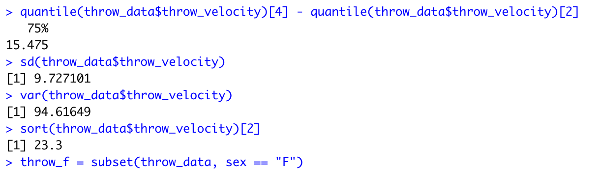
With our throw_data, find:
- Interquartile range of the throw velocities(3rd quartile - 1st quartile)
- Sd(standard deviation),var(variance) of the throw velocities
- 2nd smallest throw velocity
- Subset with sex == “F” stored in a variable called "throw_f"
Basic Charting and Plotting
R has the ability to provide us with useful plots regarding our data. There are many different ways that we can plot our data in R using some default plotting functions provided to us already.
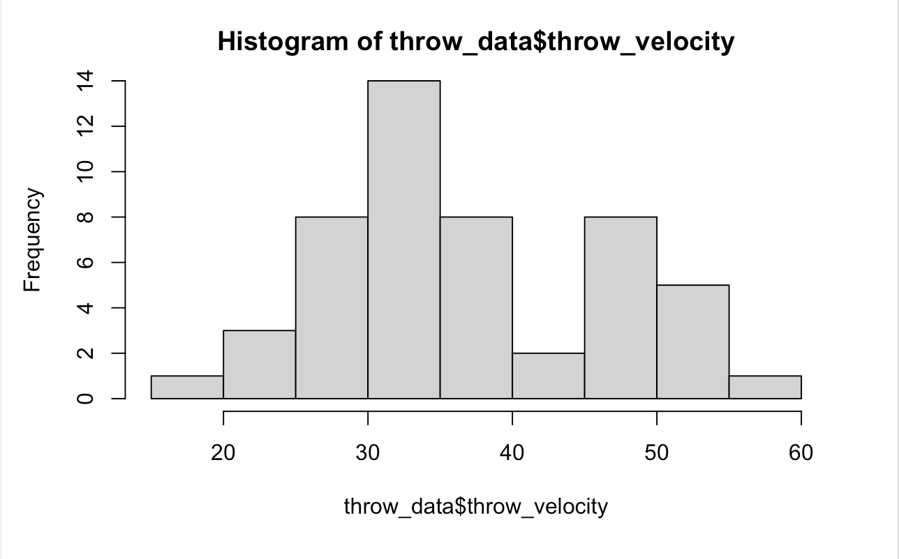
Histogram
A histogram gives us a bar chart that shows us the frequency distribution of our dataset. A histogram groups numbers into ranges and the height of each bar shows us the number of items that fall into that specific range.The hist(x) function provides us with a histogram of the data in a vector x. The command hist(throw_data$throw_velocity) gives us a histogram for the throw velocities.
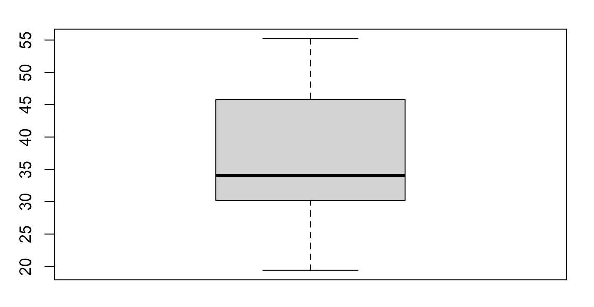
Boxplot
A boxplot shows us a graphical representation of the quartiles for our range of data. Boxplots can be useful to understand the distribution of data within our dataset. We can use the boxplot() function to create a boxplot in R.
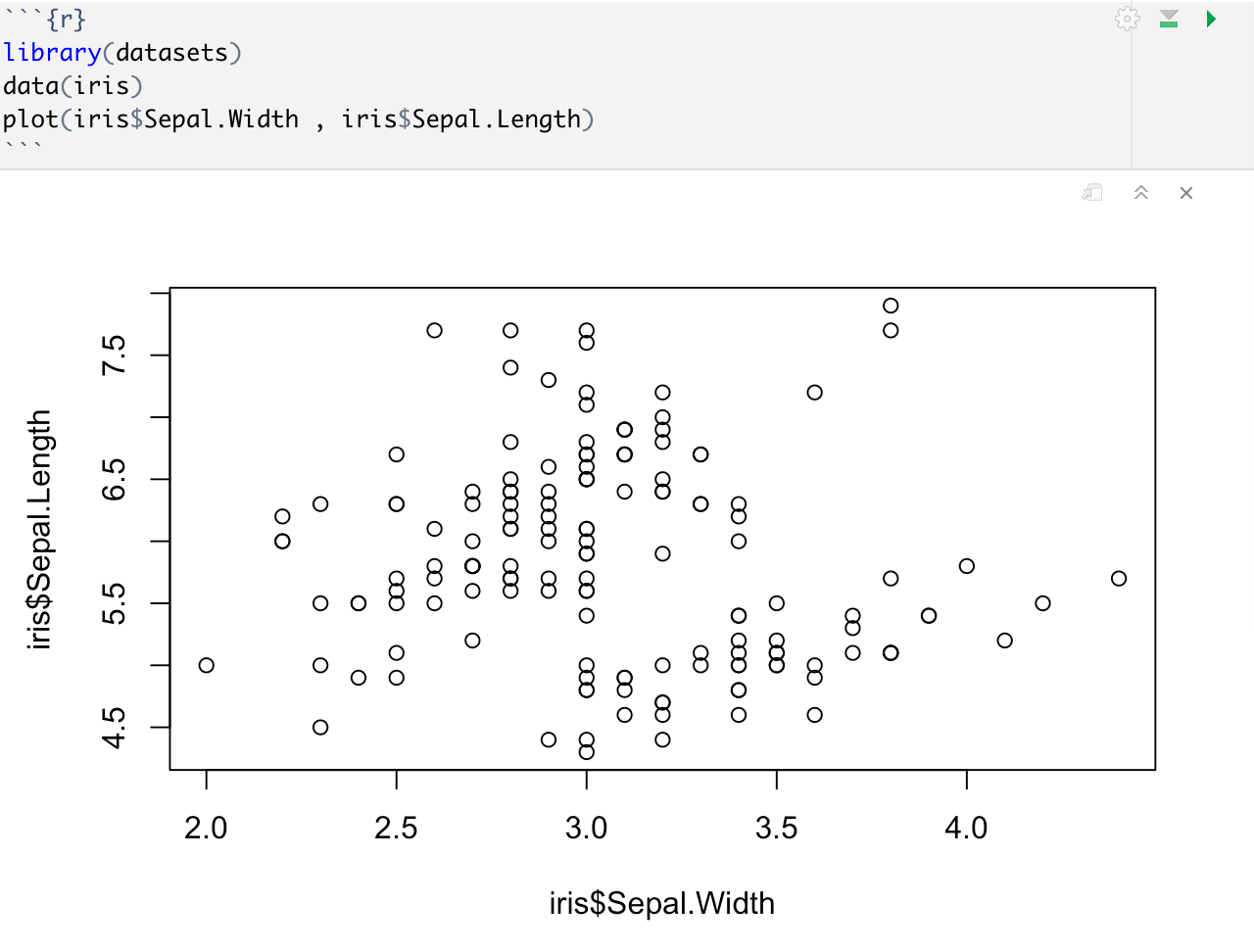
Scatter Plot
A scatterplot has points that show the relationship between 2 kinds of data.The plot() function provides us with a generic scatter plot of our data. In order to make a basic scatter plot, we can use the plot(x,y) syntax where x and y are vectors with the respective x-y coordinates for our plot.
Unfortunately, our throw_data does not lend itself to a scatter plot so we are going to import a dataset from a library in R.
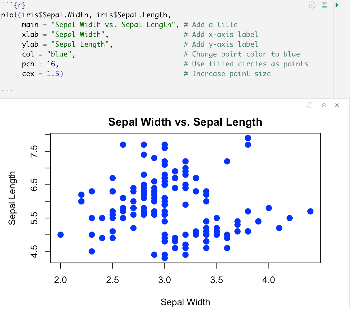
While the graphs we have created so far are functional, they may not be visually appealing. However, we can enhance our graphs by using additional parameters in our R functions. In R, functions are denoted by parentheses (), and most functions have extra parameters that can be used to customize their output. These parameters allow us to tweak various aspects of the graph, such as colors, fonts, axis labels, and more.
To view all the available parameters for a function, we can refer to its help documentation. For example, let's consider the scatter plot function. We can access its help documentation by typing ?plot or help(plot) in the R console, which will display a detailed list of all the available parameters for the plot() function. By using these parameters and adjusting their values, we can create more visually appealing and customized graphs that better suit our data visualization needs.
For example, here is our same scatter plot with some minor upgrades:
Activity 2: Working through the RMD
For some hands-on practice, you will walk through and complete the rest of the problems in the class RMD file.
Conclusion
Congratulations! You have completed our workshop on using R and RStudio for data analysis. We hope you have gained valuable insights into the power and versatility of R and RStudio for analyzing and visualizing data.
If you are interested in diving deeper into data manipulation and graphing with R, we encourage you to sign up for our R2 workshop. This advanced workshop focuses on using popular packages like ggplot2 and dplyr for creating visually appealing and informative visualizations, as well as advanced data manipulation techniques.
For those of you who are here because of classes, we want to remind you about our Ask A Trainer (AAT) appointments. Our experienced trainers are available to provide additional support and guidance whenever you need it throughout the semester. Don't hesitate to reach out for assistance with any questions or challenges you may encounter while working with R and RStudio.
Thank you for participating in our workshop, and we wish you success in your future data analysis endeavors using R and RStudio!